Benchmark Problem #1

Lloyd and Stansby (1997) performed experiments using shallow flows around submerged conical islands with small side slopes. The geometry used in the experiments and inflow and outflow conditions were very simple. However, the flow becomes complex as, on the top of the island, the water surface and velocity varied rapidly and a vortex street was generated at the lee side of the island. In addition, they observed strong vertical mixing just downstream of the apex of the island. As mentioned above, the experimental setup was simple: a conical island was installed 5.0 m downstream of the inlet in a channel 9.75 m in length and 1.52 m in width, and a steady discharge was released at the upstream boundary. The channel and the island were made of marine quality plywood and aluminium, respectively, and the channel bottom was painted to produce uniform surface roughness. More details of the experiments are described in Lloyd and Stansby (1997):

Lloyd, P.M., Stansby, P.K., 1997. Shallow water flow around model conical island of small slope. II: Submerged. Journal of Hydraulic Engineering, ASCE 123 (12), 1068-1077.
[local pdf]

Note that discussion of the roughness coefficient for this experimental setup can be found in more detail in the first paper (Experimental Arrangement section):

Lloyd, P.M., Stansby, P.K., 1997. Shallow water flow around model conical island of small slope. II: Submerged. Journal of Hydraulic Engineering, ASCE 123 (12), 1057-1067.
[local pdf]

While there are many controlled experimental datasets looking at the wake behind a cylinder, there are very few that examine the wake behind a sloping obstacle in the context of shallow water flow. As the obstacle (the island) remains submerged at all times, the wake is physically generated through a spatially variable bottom stress (i.e. gradients in bottom friction). The aim of this benchmark is to test a models ability to generate a separation region and the resulting oscillatory wake for an idealized and simplified case.

DOWNLOAD DATASET: all_data.zip

SETUP:

We will use test case SB4_02 in the Lloyd and Stansby Part II (L&S) paper (See Table 1). The steady discharge velocity is U = 0.115 m/s, water depth is h = 0.054 m, and the Reynolds number of the mean flow is Re = 6210. The ratio of the water depth to the island height (h/hi in the L&S paper) = 1.10.

Bathymetry (in "bathy" directory)

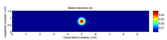
The information provided in the the Part I paper can be used to generate the bathymetry. Specifically, a conical island is placed on a flat bottom, where the water depth is 0.054 m on the flat bottom. The side slopes of the conical island are ~8 degrees, and the ratio of the water depth to the island height (h/hi in the L&S paper) = 1.10. The height of the island is 0.049 m and the diameter at the base of the island is 0.75 m. The island does not end in a point; the top section of the island is flattened, as shown in the image from the Part I paper below. This configuration can be plotted using the included "plot_bathy.m" script.

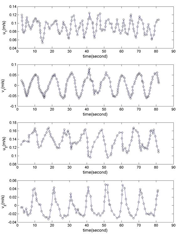
Velocity Measurements (in "comparison_data" directory)

For this benchmark, we will compare the horizontal components of velocity at two different locations behind the island. A plot of the locations and the data is shown below, as created by the plot_data.m script. Note that this data has been digitized from Figure 6 in the L&S paper. Point (1) is located along the centerline of the tank, 1.02 m behind the center of the island. Point (2) is located at the same x-location as Point (1), but 0.27 m offset in the positive cross-tank (y) direction (see image below for approximate locations).

Modelers are to provide results for at least three different numerical configurations:

1) Simulation result with dissipation sub-models included, using the roughness information included in the paper to best determine the friction factor. In the papers, the friction factor is estimated to be 0.006 (as a dimensionless pipe-flow-like drag coefficient) or a Mannings n value of 0.01 s/m^1/3. If a RE-dependent friction factor formulation is used, then a roughness height, k_s, of ~1.5e^-6 m should be used.

2) Simulation results with optimized agreement based on tuning of dissipation model coefficients (e.g. friction factor). Note that this simulation can be skipped if the modelers do not wish to optimize their comparisons.

3) Simulation result with ALL dissipation sub-models NOT included (e.g. a physically inviscid simulation). The purpose of this test is to understand the relative importance of physical vs numerical dissipation for this class of comparison.