Benchmark Problem #2
This is a field dataset - a recording of the Japan 2011 tsunami in Hilo Harbor, Hawaii. While modelers will of course aim to achieve the best agreement with the measured data, this is not the primary goal of this exercise. Here, we aim to understand the importance of model resolution and numerics on the prediction of tsunami currents:
What level of precision can we expect from a model with regard to modeling currents on real bathymetry?
Will a model converge with respect to speed predictions and model resolution?
What is the variation across different models, using the same wave forcing, resolution, and bottom friction?
To attempt to most clearly answer these questions, this field case will be somewhat idealized, or reduced in complexity, to give the modeling results the best chance of an "apples-to-apples" comparison of shallow water, tsunami currents.
For this benchmark, we will compare free surface elevation (from tide stations) and velocity information (from ADCPs). Data for this benchmark test has been provided by Randy LeVeque and Fai Cheung, who have both examined this location in the following publications:
Arcos, M and
LeVeque, R. (2014) Validating Velocities in the GeoClaw Tsunami Model using
Observations Near Hawaii from the 2011 Tohoku Tsunami. http://arxiv.org/abs/1410.2884
[local pdf]
Cheung KF, Bai
Y, Yamazaki Y (2013) Surges around the Hawaiian islands from the 2011 Tohoku
tsunami. J Geophys Res 118:5703{5719, DOI 10.1002/jgrc.20413
[local pdf]
DOWNLOAD DATASET: all_data.zip
SETUP:
Bathymetry (in directory "bathy"):
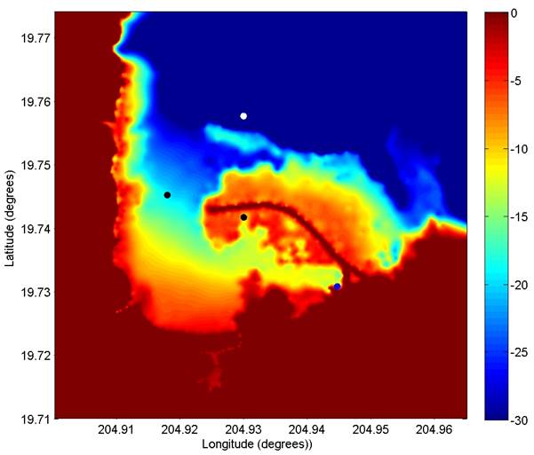
The figure below (the bathymetry data) can be plotted in Matlab with the "plot_bathy.m" script. The data is provided in (lat,long) on a 1/3 arcsec grid. Note that shown on this figure are also the simulation control point (white dot), the two ADCP locations (black dots) and the tidal station (blue dot). As mentioned above, this problem has been "reduced" in an attempt to isolate differences in the employed incident wave forcing. For the bathymetry data, this "reduction" manifests as a flattening of the bathymetry at a depth of 30 meters; in the offshore portion of the bathymetry grid, there are no depths greater than 30 m.
Incident Wave (in directory "incident wave")
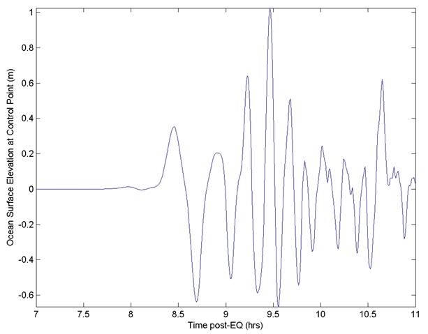
For this case, modelers are asked to drive their simulations with an offshore simulated free surface elevation time series (the "control point"). The location of this time series is (lat,long)= [19.7576, 204.93]. Modelers may force their simulations in whichever way is convenient (e.g. through upper grid boundary, or with an internal source generator in the northern part of the domain), but should check with their modeled time series at the control point to ensure that they are generating the proper offshore wave condition. The control-point ocean-surface-time-series can be plotted using the "load_offshore_wave.m" script, which will create the figure below.
Note that the above simplification will lead to a physical mismatch between the simulated and actual data; as the incident wave will vary spatially (albeit weakly) as it approaches the harbor. Modelers are of course encouraged to simulate the complete problem with their models (from source to harbor with nesting), but this is optional.
Benchmark Data(in directory "comparison data")
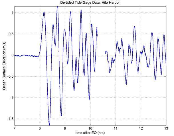
Free surface elevation data at the
tidal station
The
first comparison will be to check the water surface elevation at the tidal
station:
Hilo Tide Station: [lat, long]=( 19.7308, 204.9447 )
The script (load_plot_tidegage.m) will load and plot the 1-minute de-tided gage data (de-tiding of raw data done by Randy LeVeque). Modelers should shift the simulated and tidal data such that the leading numerical wave arrives at the proper time, and this time shift should be used in the velocity comparisons. The tide gage data is shown below.
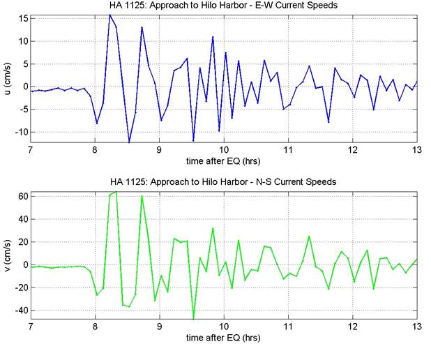
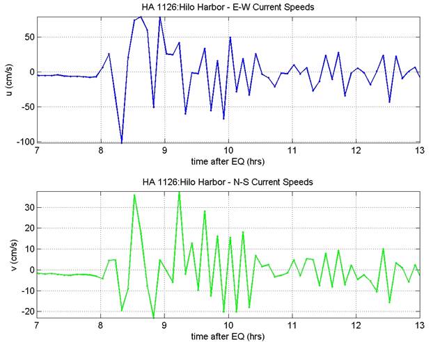
Depth-Averaged Horizontal Velocity
data at ADCP locations
The
official locations of the ADCPs are:
HA1125, Harbor Entrance: [lat, long] = (19.7452, 204.9180)
HA1126, Inside Harbor: [lat, long] = (19.7417, 204.9300)
The processed ADCP data can be loaded & plotted with the "load_plot_adcp.m" script, and is shown in the images below. This data has been averaged over the depth, and then filtered to remove long-period tidal components. Modelers who wish to examine the raw data may use the following data pages, constructed by Randy LeVeque:
http://coastal.usc.edu/currents_workshop/problems/HAI1125_Hilo/plots.html
http://coastal.usc.edu/currents_workshop/problems/HAI1126_Hilo/plots.html
Modelers are requested to provide results for at least three different numerical configurations:
1) Simulation result at ~20 m resolution (2/3 arcsec, de-sample the input bathymetry), using a Mannings n coefficient of 0.025 (or approximate equivalent if using a different bottom stress model)
2) Simulation result at ~10 m (1/3 arcsec) resolution using a Mannings n coefficient of 0.025 (or approximate equivalent if using a different bottom stress model)
3) Simulation result at 5 m resolution (1/6 arcsec, or the lowest resolution possible; use bi-linear interpolation), using a Mannings n coefficient of 0.025 (or approximate equivalent if using a different bottom stress model)
Modelers are encouraged to compare simulation results both locally (required by the benchmark) as well as to examine statistical measures of spatial variability between the different resolutions.