Benchmark Problem #4

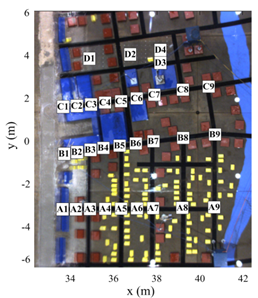
This experiment has a single long-period wave (NOT a solitary wave) propagating up a piecewise linear slope and onto a small-scale model of the town of Seaside, Oregon. Free surface information was recorded via resistance-type wave gauges and sonic wave gages. Velocity information was recorded via ADV's.

Complete details of the experiment can be found in the accompanying journal paper:

Park, H., Cox, D., Lynett, P., Wiebe, D., and Shin, S. (2013) "Tsunami Inundation Modeling in Constructed Environments: A Physical and Numerical Comparison of Free-Surface Elevation, Velocity, and Momentum Flux." Coastal Engineering, v. 79, pp. 9-21, doi: 10.1016/j.coastaleng.2013.04.002. [local pdf]

For video from similar model trials, see this video: https://www.youtube.com/watch?v=nj98sHcTGOo

For this benchmark, we will compare free surface, velocity, and momentum flux information recorded throughout the tank.

DOWNLOAD DATASET: all_data.zip

SETUP:

Water depth @ Wavemaker: 0.97m

Incident Wave (in directory "incident wave")

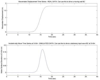
The generated wave for this problem is not a solitary wave. It is custom wave meant to maximize the stroke of the wavemaker, while generating a long period wave. Note that due to this generation approach, the wave is not permanent, like a solitary wave. Numerically, the wave can be generated using two different methods:

1) The wavemaker displacement time series can be used if a moving wall boundary condition is available in the numerical model.

2) The time series of incident wave elevation at X=5m can be used to force the numerical model at X=5 m. Note that this is a synthetic time series, based on simulation with a moving wall boundary condition.

Both of these time series can be seen and plotted using the "load_wavemaker_motion.m" script in the "incident_wave" directory (see image below).

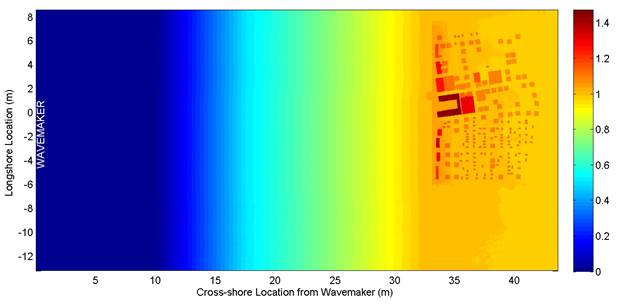
Bathymetry (in directory "bathy"):

Figure below (the bathymetry data) can be plotted in Matlab with the "plot_bathy.m" script.

Benchmark Data (in directory "comparison data")

The following data should be compared with the numerical model output.

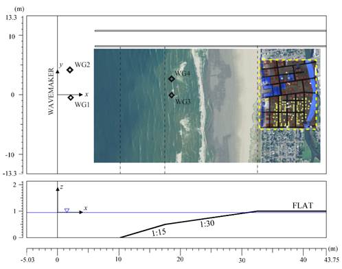
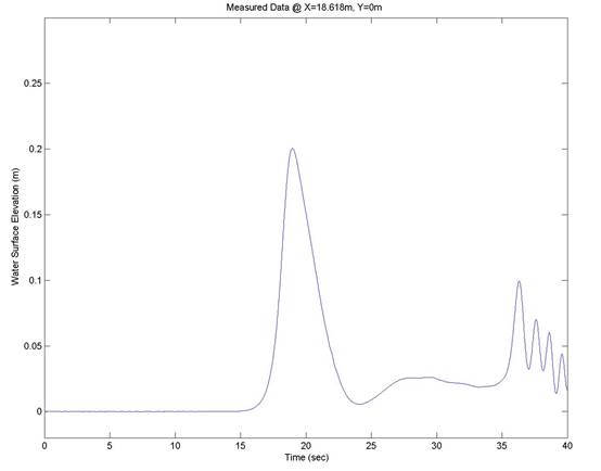
Free surface elevation data at WG3
This data is contained in the file: "Wavegage.txt", and can be plotted with the script load_WG3.m. The location of the wave gage is shown below (see also included journal paper). Note that there is other data included in these files as well. Modelers may compare with any data they wish, but please be sure to show comparisons at WG3. Comparisons at this particular location will be used to ensure that the generated waves in the model are correct, in terms of amplitude, period, and arrival time.

	X(m), Y(m)
Wmdisp Wmwg (At the wave maker)	0, 0
Wg1	2.068, -0.515
Wg2	2.068, 4.065
Wg3	18.618, 0
Wg4	18.618, 2.86

Overland Flow Depth, Cross-shore (x-direction) Velocity, and cross-shore Specific Momentum Flux
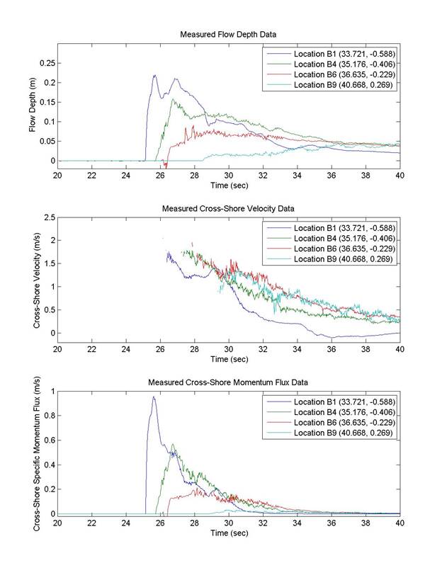
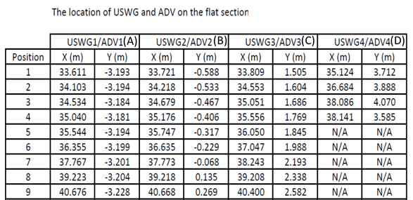
This data comparison is the primary comparison of the benchmark exercise. Here, we compare flow depth (H), velocity (u), and specific momentum flux (Hu²) at four locations: B1, B4, B6, B9 (see image and table below). These four locations are discussed in depth in the journal article linked above. Data for these locations can be plotted with the script "load_B1_4_6_9.m." The data is shown below. Note that there is data for other overland flow locations included as well (in "comparison_data/other"). Modelers may compare with any data they wish, but please be sure to show comparisons at B1, B4, B6, and B9.